 PhotonSharp
System requirements
PhotonSharp runs in a browser. These are practical minimums for editing and simulating small projects; larger circuit graphs can need more memory and a wider display.
| Requirement | Practical minimum |
|---|---|
| Computer | Desktop or laptop with a dual-core CPU and 4 GB of RAM. 8 GB or more is recommended for large graphs and several open tabs. |
| Display | 1280 × 720 pixels for the full editor. Documentation works on smaller screens, but the circuit canvas is easier to use with more space. |
| Browser | A current Chrome, Edge, Firefox, or Safari release with JavaScript, cookies, and browser storage enabled. The optional Python Tools extension also needs Web Workers. |
| Connection | An internet connection for saving projects and server-side compilation and simulation. Browser drafts are stored locally until you save. |
| Graphics | No dedicated GPU is required on your computer. Vulkan acceleration is an optional server-side compute choice when available. |
Storage: A free account includes 250 MB of saved project space. This is cloud project storage, not a requirement for free disk space on your computer.
Your first circuit
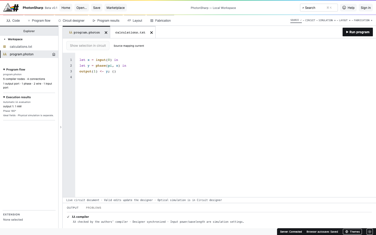
Open PhotonSharp, create a project, and select program.photon in Explorer. This is the active λλ source file. The small starter program below reads an optical input, changes its phase, and sends it to an output:
let light = input(0) in
let shifted = phase(pi, light) in
output(1) <- shifted;
()
Paste the program into Code. A valid edit updates the generated circuit. The names describe signal flow; the compiler creates the components and wires.
Tip: Use Open → Examples for a starting design. The legacy calculations.txt file is a separate matrix calculator; it is not the λλ circuit source.
Know the workspace
Code and Program Flow
Code is where you edit λλ expressions. Program Flow shows the compiler’s interpretation of their inputs, operations, and outputs. Click a node to inspect it.
Circuit Designer
Choose a .photon file in Explorer, then open Circuit Designer. The canvas shows the generated components and connections; use Fit to view for a large graph.
Program Results
Run program evaluates ideal λλ output fields. Use this view for output power, phase, and complex amplitude.
Layout and Fabrication
These views support geometry review and process preparation. They do not replace foundry design-rule checks or approval.
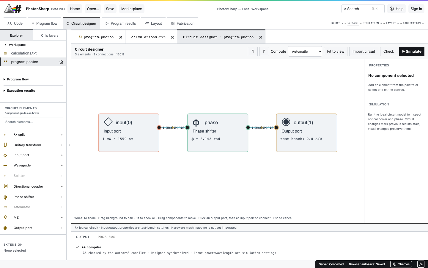
In the designer, choose a component to inspect its properties. The left palette provides component guides on hover. You can move components and edit supported properties; valid designer changes regenerate λλ expressions.
Run and inspect the response
- Run program in Code or Program Results. Read the ideal outputs and any syntax or signal-use errors.
- Simulate in Circuit Designer for component readings such as optical power and phase. Choose Automatic, CPU, or Vulkan where available.
- Choose Vulkan GPU when available. In Circuit Designer, use the Compute menu, then Simulate. The result reports the actual GPU and float32 precision, or explains a CPU fallback. Automatic keeps small jobs on CPU to avoid GPU startup overhead; batches of 32 or more independent cases can use Vulkan. GPU selection is pinned by the server administrator. Spectral analysis remains a separate CPU solver.
- Change one parameter, such as
phase(pi, light)tophase(pi / 2, light). Run again and compare the output phase.
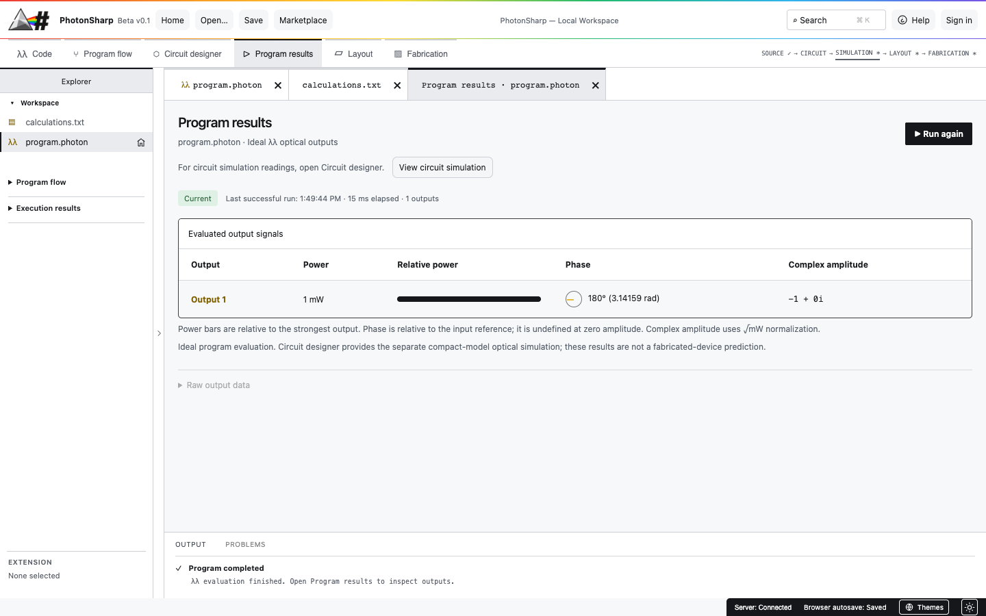
At zero amplitude, phase is undefined. The compact model is coherent and forward-only; it does not model noise, timing, reflections, or physical fabrication variation.
Build a one-bit optical ALU experiment
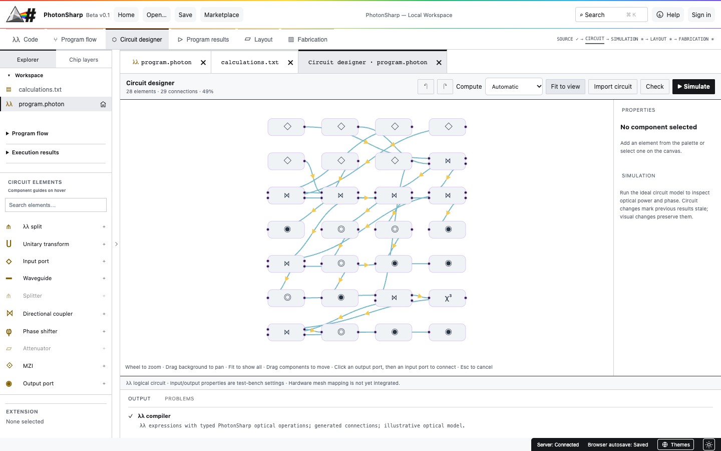
Start with a small, testable target: inputs A, B, and carry-in Cin; measurements labeled AND, OR, XOR, SUM, and COUT. The downloadable example is a λλ program that compiles into 28 components and 29 inferred connections. Its thresholds are test measurements, while operation selection remains outside the optical circuit.
- Define the encoding. Treat zero and 1 mW as candidate binary input powers. Fix relative input phases and wavelength. Document these choices before interpreting a measured bit.
- Split and mix the signals. Add
sourcevalues, vacuum inputs, andcoupleroperations. Useunpackfor each two-output component and consume both outputs. - Add measurement points.
probe(threshold_mw, signal)records a threshold bit and passes the same optical signal onward. Usedetect(responsivity, signal);oroutput(port) <- signal;for final consumption. - Compile and inspect. Paste the example into a selected .photon file. Open Circuit Designer, choose Fit to view, then Check and Simulate. Every connection comes from the expressions.
- Test every input. Change the A, B, and Cin source powers through all eight 0/1 combinations. Record AND, OR, XOR, SUM, and COUT probe bits and compare them to the truth table below.
- Stress the model. Vary power, phase, and thresholds. A nominal truth-table pass alone does not establish robust logic, regenerated carry, or on-chip operation selection.
| A | B | Cin | AND | OR | XOR | SUM | COUT |
|---|---|---|---|---|---|---|---|
| 0 | 0 | 0 | 0 | 0 | 0 | 0 | 0 |
| 0 | 0 | 1 | 0 | 0 | 0 | 1 | 0 |
| 0 | 1 | 0 | 0 | 1 | 1 | 1 | 0 |
| 0 | 1 | 1 | 0 | 1 | 1 | 0 | 1 |
| 1 | 0 | 0 | 0 | 1 | 1 | 1 | 0 |
| 1 | 0 | 1 | 0 | 1 | 1 | 0 | 1 |
| 1 | 1 | 0 | 1 | 1 | 0 | 0 | 1 |
| 1 | 1 | 1 | 1 | 1 | 0 | 1 | 1 |
Scope of the result: The example’s ideal model passes these eight nominal cases. The probe bits are external measurements, not regenerated optical Boolean outputs. The design does not yet implement an optically selected, cascaded, fabrication-ready ALU.
Save and share your work
Browser autosave preserves a draft in this browser. Choose Save to update the project on the server. Signed-in accounts can save projects across devices and use project sharing. Before an MCP client edits a project, save your browser changes; afterward, load the newer saved version. Keep generated connection configurations private.
The Extended λλ Toolset and MCP Server are first-party workspace extensions. Open Marketplace to enable or disable them, and use View Extension Help for individual component details.
From circuit to layout review
Open Layout to generate and inspect review geometry. Unresolved device outlines require physical implementations. In Fabrication, import process specifications, review the layer stack and checks, and export a review package. The review ZIP includes a generic KLayout width/spacing runset that you can run locally with klayout -b -r generic-review.drc. Its GDSII file can also be examined with GDSFactory and an open PDK. These tools do not supply calibrated device cells or a foundry rule deck by themselves. PhotonSharp’s current outputs are not foundry-qualified; a process design kit, full design-rule and physical verification, and foundry approval remain necessary.
When something does not open or compile
“Select a valid .photon file!”
Select a .photon file in Explorer before opening Circuit Designer, Layout, or Fabrication. Other workspace files can still be opened in Code.
Unused or duplicated signal
Each optical signal is linear: consume it once. Use unpack for two-output operations and terminate every branch at an output or detector.
Old circuit after MCP edits
Save your browser draft, then reload the saved project after the MCP client finishes. Browser drafts are not live-synchronized with remote edits.
Simulation differs from hardware
The model uses idealized optical operations. Check phase, loss, thresholds, noise sensitivity, process parameters, and measurement assumptions before drawing physical conclusions.
Wavelength, reflections and feedback
Open Circuit Designer → Spectral analysis. The original ideal λλ evaluator remains available. The separate linear scattering solver propagates reciprocal optical fields and solves feedback simultaneously with a sparse complex128 CPU solver. It supports up to 2,000 components, 8,000 physical ports and 201 wavelength samples, subject to budgets of 250,000 port-samples and 50,000 component-samples.
- Leave Setup on Automatic · use my circuit and click Run analysis. The source wavelength sets the reference and a ±50 nm sweep (bounded to the supported range); sample count is automatically reduced for larger circuits. Choose At my source wavelength for one reading, or Custom settings to edit the range and temperature change. Multiple source wavelengths are flagged; the lowest is used as reference and sources remain phase-locked. A detector power trace is selected automatically when available.
- Open Advanced settings → Material and reflection coefficients to supply group index, thermo-optic dn/dT, linear expansion, and power reflectance. The UI applies these values to all waveguides for this run; MCP can provide separate values per waveguide.
- Run analysis, select a readout, and download the complete JSON for comparison. Analysis does not change source, circuit parameters or saved projects.
The first-order index model is n_eff(λ,T) = n_ref + (n_ref − n_group)(λ − λ_ref)/λ_ref + (dn/dT)ΔT. Length is scaled by 1 + αΔT. Supply coefficients appropriate to your material and wavelength interval. Zero thermal coefficients mean no thermal sensitivity. Couplers and phase shifts remain ideal, wavelength-independent elements. Reflection is a specified passive waveguide two-port model, not a prediction from geometry. Unconnected ports are matched terminations. Nonlinear Kerr, transient timing, noise, electromagnetic field solving, spatial thermal solving and process Monte Carlo are not included.
For a feedback test, connect coupler output 2 through an attenuator back to input 2, connect a source to input 1 and a detector to output 1. The spectral solver supports this graph; the expression compiler and original forward solver do not support feedback source programs. A lossless disconnected resonant loop may be singular and is rejected.
Generate cells and run polygon checks
Open Layout → Generic PDK layout. This separate adapter uses GDSFactory's generic SOI development process to generate supported straight waveguides, directional couplers, splitters, phase heaters and MZI cells, then route their optical ports. Sources/detectors become external optical interfaces. The first release supports 32 components and 100 connections, with no automatic feedback routing or custom multilayer stack mapping.
The generic process, component mapping, routing and checks are selected automatically; no process form is required. Click Generate physical geometry and inspect the red KLayout polygon violation markers. The precheck covers WG minimum width 0.4 µm and space 0.2 µm only. Export GDSII or OASIS plus the process/DRC report. Exported geometry is for development and review: generic cells are not calibrated to your logical phase/coupling parameters, and passing these checks is not a full foundry DRC/LVS signoff. Unsupported nonlinear devices are rejected rather than represented as fabricated devices.