PhotonSharp
What a .photon program describes
A λλ program describes how optical signals move through operations. Each expression consumes its input signal and produces a new value. The compiler generates components and wires from that flow. You do not specify canvas coordinates, component IDs, or connect() calls in the source.
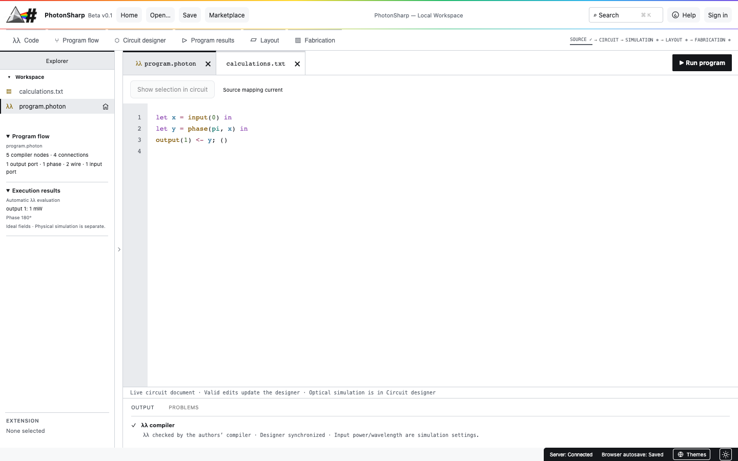
Start by editing program.photon in the Code tab. The program is the source of the generated circuit; canvas positions and chip-layer metadata are kept separately. The current evaluator is an idealized optical model, not a foundry process simulation.
Reading path: Sections 02–06 teach the core language with no extended tools. Sections 07–08 add PhotonSharp optical operations. Use the searchable API reference for signatures, units, return types, and valid ranges.
Your first program
// One input, one phase shift, one output.
let light = input(0) in
let shifted = phase(pi, light) in
output(1) <- shifted;
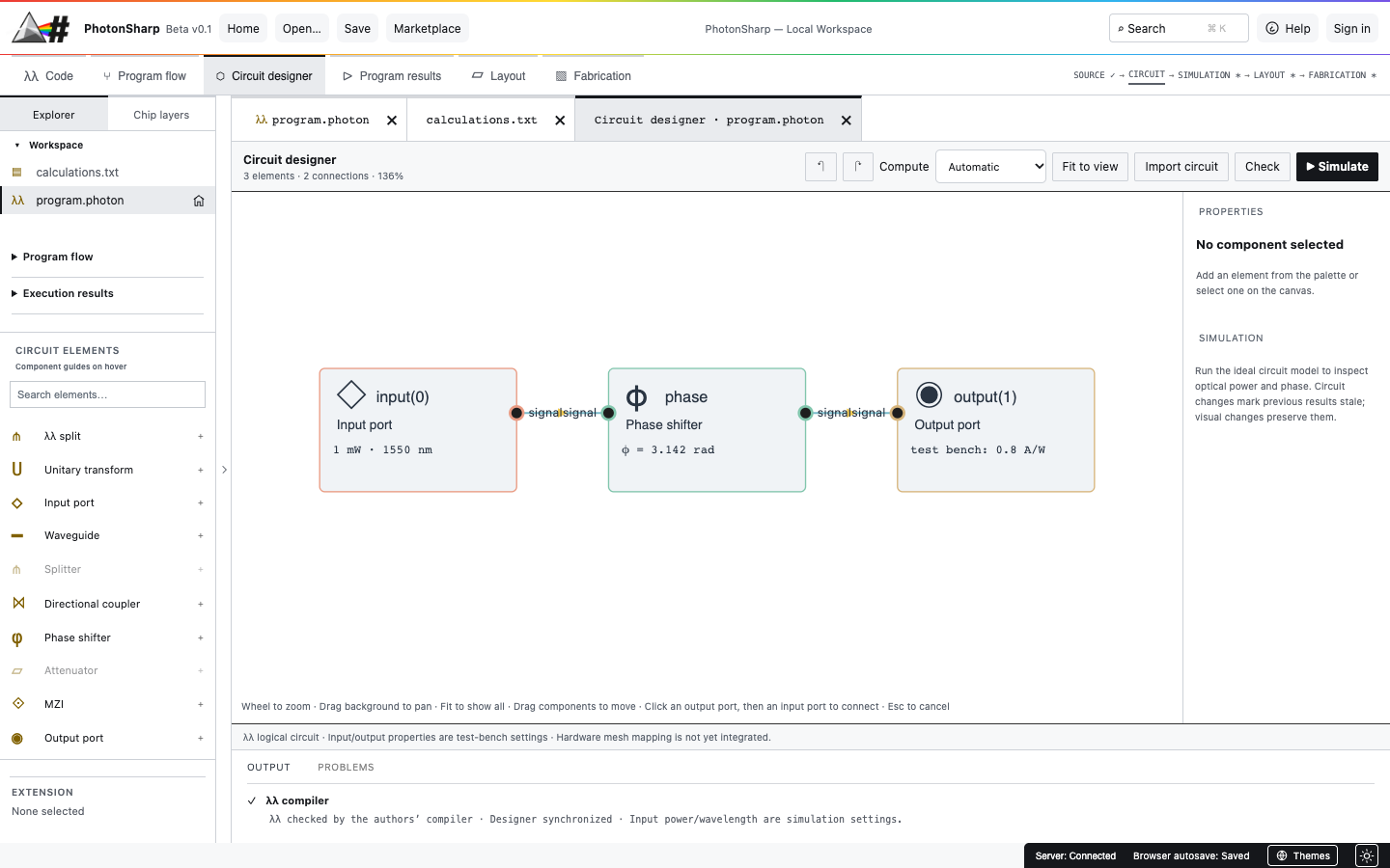
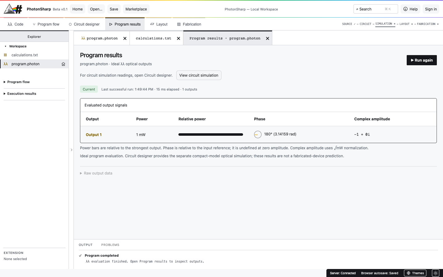
()input(0)creates an optical input at port 0. The ideal test bench defaults to 1 mW at 1550 nm.let light = … ingives the resulting signal a name for the rest of the expression.phase(pi, light)consumeslightand returns a signal shifted by π radians.output(1) <- shifted;consumes the final signal at output port 1.()is the Unit value that ends the program.
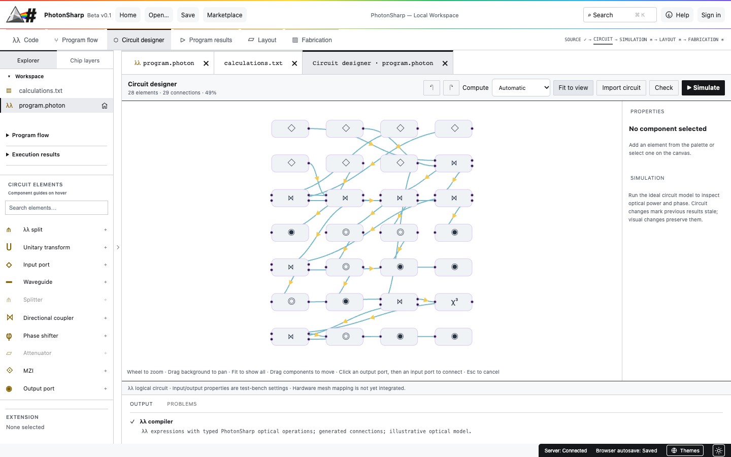
Click Run program for ideal output readings. Open Circuit Designer to see the inferred graph. If you edit the source, the graph is regenerated from the new signal flow.
How expressions are written
| Form | Purpose |
|---|---|
let name = value in body | Bind one value and continue in the body. Nest bindings to build a chain. |
unpack pair as (a, b) in body | Give both signals from a two-output operation separate names. |
(a, b) | Supply an ordered optical pair to a two-input operation. |
output(port) <- signal; body | Consume a signal at a numbered output and continue. |
() | Unit value, normally the end of the program. |
Names begin with a letter or underscore and then contain letters, digits, or underscores. Port numbers are nonnegative integers. Whitespace and line breaks separate tokens but do not define blocks. Comments start with // or # and run to the end of a line.
Numeric parameters
Write decimal or scientific notation, such as 0.5, -1, or 1e-3. pi and π are equivalent. Parameter expressions allow multiplication and division, for example pi / 2 or 2 * pi. The parameter parser does not implement general addition, subtraction, or numeric variables; calculate those values before inserting them into the source. Parameters must be finite.
Operations use positional arguments. The language currently has no imports, user-defined functions, classes, methods, loops, or conditionals. For a complete alphabetical inventory of the actual surface, use the API reference.
Types and the one-use signal rule
The main types are Optical (one signal), (Optical, Optical) (a pair of signals), Real (a numeric literal or parameter), and Unit (() or a consuming operation). A signal is linear: after an operation uses it, that name cannot be used again. Every produced optical signal must reach exactly one consumer.
// split creates two new signals; both must be consumed.
let light = input(0) in
unpack split(0.5, light) as (upper, lower) in
output(1) <- upper;
output(2) <- lower;
()
The two branches are not references to the same signal. If you need another branch, use another two-output operation. Do not reuse light after split, and do not leave lower unused. Each input(port) and output(port) number must be unique within a program.
The complete core operation set
| Operation | Signal flow | What it computes |
|---|---|---|
input(port) | none → Optical | Read one test-bench optical input. |
phase(radians, signal) | Optical → Optical | Rotate the complex field by the given angle. |
split(ratio, signal) | Optical → pair | Core amplitude split: fields become ratio × E and (1 − ratio) × E. At 0.5, each output has one quarter of the input power. |
unitary(matrix, (a, b)) | pair → pair | Apply a 2×2 unitary transform. Matrix can be H, I, or an explicit 2×2 matrix. |
output(port) <- signal; | Optical → consumed | Expose one optical output for evaluation. |
For an explicit matrix, write [[a, b], [c, d]]. Entries can be real numbers or complex(real, imag). The compiler rejects a matrix that is not unitary. The built-in H is the normalized Hadamard matrix; I is identity.
Two inputs through a unitary
// H mixes two optical inputs and produces two outputs.
let a = input(0) in
let b = input(1) in
unpack unitary(H, (a, b)) as (upper, lower) in
output(2) <- upper;
output(3) <- lower;
()
Both inputs are consumed by the pair, and unpack names both results. Change one input’s phase to see how coherent fields interfere. This is still core λλ; no extended component is required.
Use the extended toolset
PhotonSharp adds typed optical operations to the same expression syntax. Enable Extended Lambda Lambda Toolset in Marketplace for a workspace; new projects include it by default. You still write signal expressions, and the compiler still infers components and connections.
| Operation | Signal flow | Purpose |
|---|---|---|
source(power_mw, phase_rad) | none → Optical | Create a coherent model source. Zero power supplies a vacuum input. |
waveguide(length_um, loss_db_cm, effective_index, signal) | Optical → Optical | Apply propagation phase and distributed loss. |
attenuate(loss_db, signal) | Optical → Optical | Apply lumped optical loss. |
kerr(gamma, signal) | Optical → Optical | Apply illustrative power-dependent phase; optional loss_db can be inserted before the signal. |
power_split(ratio, signal) | Optical → pair | Split by power fraction, unlike core split. |
coupler(ratio, (a, b)) | pair → pair | Mix two coherent fields with an ideal directional coupler. |
mzi(phase_rad, coupling_ratio, (a, b)) | pair → pair | Model a two-coupler Mach–Zehnder interferometer. |
probe(threshold_mw, signal) | Optical → Optical | Record a threshold bit while passing the optical signal onward. |
detect(responsivity_a_w, signal); | Optical → consumed | Terminate a signal and report modeled photocurrent. |
Two kinds of split: split(0.5, E) yields fields of 0.5 E each, so each has 25% of input power. power_split(0.5, E) yields fields of approximately 0.707 E, so each has 50% of input power. Both require unpack and two consumers.
probe produces a measurement bit, not a new Boolean optical signal. detect ends the optical path. All parameter units and ranges are listed in the reference table.
Mix, observe, and terminate two branches
// Two coherent sources enter a 50:50 coupler.
let a = source(1, 0) in
let b = source(0, 0) in
unpack coupler(0.5, (a, b)) as (upper, lower) in
let observed = probe(0.25, upper) in
output(1) <- observed;
detect(0.8, lower);
()
The upper branch is measured and sent to an output; the lower branch ends at a detector. Try changing b to source(1, pi / 2) to examine interference. A detector can appear before the next expression separated by a semicolon; arbitrary semicolon sequencing of live optical values is not supported.
From source to readings
- Create or open a project. Select the active
.photonfile in Explorer. The home marker identifies the program being run. - Edit and check. Enter a complete expression ending in
(). Compiler problems identify source locations. - Inspect the graph. Open Program flow for an expression overview and Circuit Designer for components and inferred wires. Use Fit to view for larger designs.
- Run the program. Program results shows ideal output power, phase, and complex amplitude. Probe and detector readings are separate model measurements.
- Review physical assumptions. Layout and Fabrication do not turn a valid λλ program into a foundry-approved mask. Choose process data and run appropriate physical checks before manufacturing claims.
Common errors and current limits
| Message or symptom | What to check |
|---|---|
| Unbound variable | A signal name was misspelled or used before its let or unpack binding. |
| Not consumed / used twice | Route every optical result once. Use unpack for both branches and end each branch with an output or detector. |
| Expected a pair / one signal | Two-input operations need (a, b); one-input operations need a single Optical value. |
| Invalid ratio or negative loss | Ratios must be from 0 to 1. Powers, lengths, losses, thresholds, and detector responsivity must be nonnegative; effective index must be positive. |
| Non-unitary matrix | Use H, I, or a valid 2×2 unitary matrix. |
| Unexpected token | Check parentheses, commas, in, the output arrow <-, and the semicolon before the next expression. |
IDE limits are 1 MB of source, 20,000 tokens, and 200 levels of expression nesting. The ideal λλ evaluator uses a single-wavelength, coherent, forward-only compact model. Circuit Designer also offers a separate Spectral analysis solver for linear scattering networks with wavelength sweeps, reflected waves, feedback, and supplied dispersion/thermal coefficients. Automatic setup detects the source wavelength and selects a bounded sample count; advanced controls remain available. Layout → Generic PDK layout automatically maps supported cells, routes optical ports and runs basic waveguide polygon checks, with GDSII/OASIS export for development review. See Advanced analysis for model scope and examples. The ideal evaluator does not model feedback, reflections, timing, noise, thermal effects, dispersion, or process variation. The separate spectral solver has its own scope described in Help. Kerr behavior is illustrative. Passing a truth table is not evidence of a fabricated device’s performance.
Study the optical ALU experiment
The complete one-bit ALU .photon file uses optical source powers for A, B, and Cin. It combines couplers, probes, detectors, and a Kerr element; the compiler generates the graph from the source. Follow the ALU walkthrough and eight-row truth table to reproduce its nominal tests.
// Excerpt only — use the complete file above to compile.
let A = source(1, 0) in
let vac_A = source(0, 0) in
unpack coupler(0.5, (A, vac_A)) as (split_A_a, split_A_b) in
// Continue consuming both branches in the full example.
The excerpt is intentionally incomplete. The full example is an idealized threshold-measurement experiment: probe bits do not regenerate optical logic levels, and operation selection remains external. The probe reference describes the exact measurement behavior.